
Freeze Panes in Excel
Work smarter, not harder!
Excel Tip – Scrolling through a large spreadsheet can be overwhelming. If you’ve ever gotten lost because you don’t know which column or row you are looking at, you know what I’m talking about. Luckily, there is a feature in Excel called “Freeze Panes” that continuously displays the headings so you will always know where you are. Use this tip to freeze the rows and columns in your spreadsheet.
Freeze Panes
- Click in the cell where the freeze is to occur – below the row(s) to freeze and to the right of the column(s) to freeze. In the example below, we want to freeze rows 1 & 2 as well as column A so we need to click in cell B3.
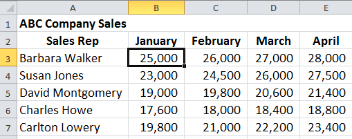
2. From the “View” tab, in the “Window” group, click the Freeze Panes button and choose Freeze Panes. The titles in rows 1 & 2 and column A will continuously display while scrolling through the spreadsheet.
> To unfreeze, on the “View” tab, in the “Window” group, click the Freeze Panes button and choose Unfreeze Panes.
Watch the video below and see how to freeze panes in Excel.
If you need help or information about the tip, contact us and we will be happy to go over it with you.